RT3D IRI Cartesian Ray Trace

Pure-Python 3D RT Workflow

Build a 3D IRI profile on a `(lat, lon, alt)` grid, run RT3D oblique fan tracing, and generate side/front plus route-aligned 3D face plots.

This page explains:

• examples/run_rt3d_iri_cartesian.py

Call Flow

1. main() parses --config and --event.
2. _run(...) loads a 3D profile:
3. RT3DProfile.from_cfg(..., fetch_iri=True, fetch_geomag=...)
4. Tracing grid is extended to ground (default):
5. extend_to_ground=true adds 0..z_floor with zero density.
6. Optional collision volume is built:
7. ComputeCollision.from_nrlmsise_3d(...)
8. on failure, zeros are used.
9. RT3D(profile=...) initializes solver state.
10. _trace_fan(...) runs all rays via:
11. RT3D.oblique_trace(...)
12. If Hamiltonian fails for most rays, script retries with gradient solver.
13. Figures are created:
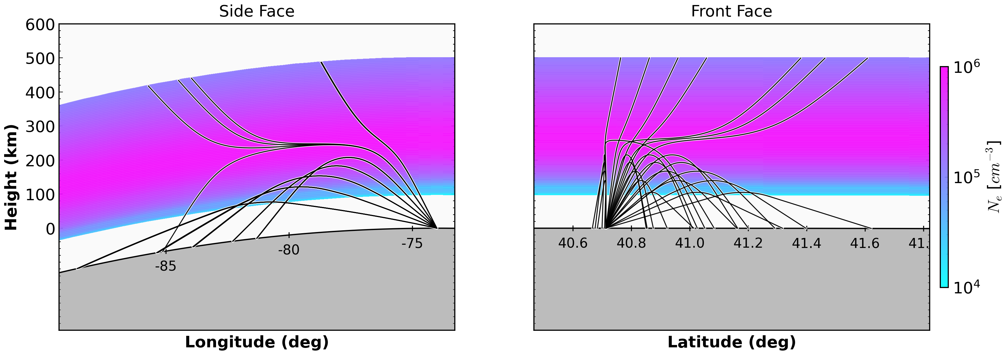
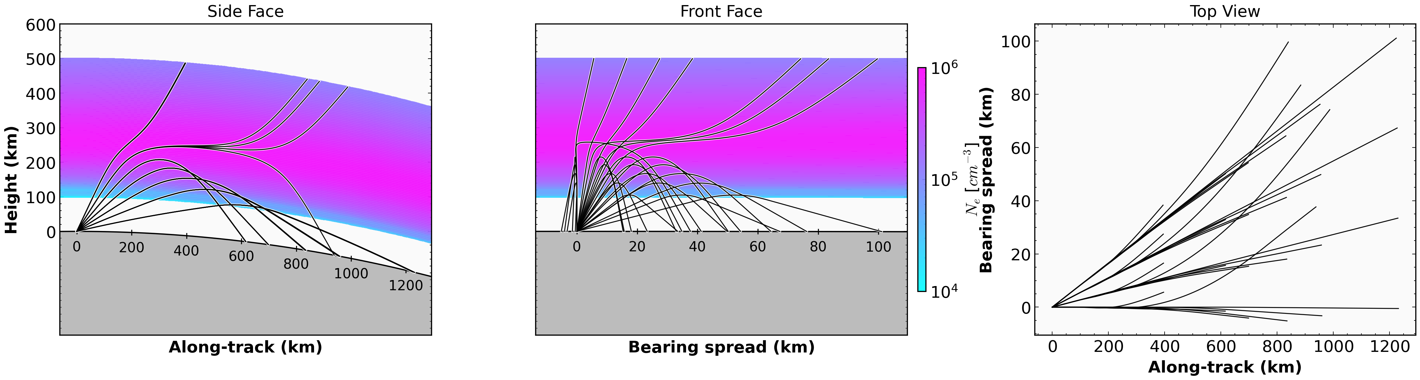
14. _plot_ray_faces(...) -> side/front in lat/lon views
15. _plot_route_faces(...) -> 3-panel route view: along-track, bearing-spread, and top view

Solver Notes

• config3D.json controls default coordinate/solver:
• use_spherical -> spherical or cartesian tracing
• solver -> "hamiltonian" or "gradient"
• The script includes robust fallback from Hamiltonian to gradient when failure ratio is high, to keep example outputs usable.

Key Code

1) Build RT3D Profile

rt_profile = RT3DProfile.from_cfg(
    cfg=cfg,
    time=event_time,
    fetch_iri=True,
    fetch_msise=False,
    fetch_geomag=fetch_geomag,
    workers=workers,
)

2) Run 3D Fan Traces

out = rt.oblique_trace(
    freq_hz=float(f_mhz) * 1e6,
    elevation_deg=float(el),
    azimuth_deg=float(az),
    coordinate_system=str(coordinate_system),
    solver=str(solver),
    x0_km=float(x0_km),
    y0_km=float(y0_km),
    z0_km=float(z0_km),
    mode="O",
    formulation="appleton-hartree",
    collision_hz=collision_hz,
    b_abs_t=b_abs_t,
    b_psi_deg=b_psi_deg,
    max_step_km=2.0,
)

3) Plot Faces

_plot_ray_faces(
    ne_grid=ne_plot,
    ray_path_data=ray_paths,
    lats=rt_profile.lats,
    lons=rt_profile.lons,
    heights=heights_plot,
    origin_lat=origin_lat,
    origin_lon=origin_lon,
    out_file=out_file,
)

and

_plot_route_faces(
    ne_grid=ne_plot,
    ray_path_data=ray_paths,
    lats=rt_profile.lats,
    lons=rt_profile.lons,
    heights=heights_plot,
    origin_lat=origin_lat,
    origin_lon=origin_lon,
    bearing_deg=bearing_ref,
    out_file=out_file_route,
)

The route-aligned panel uses PlotRays3DRouteFaces and now renders:

1. along-track vs height
2. bearing-spread vs height
3. top view (along-track vs bearing-spread)

By default, the colorbar is anchored after panel 2 and the spacing between panel 2 and panel 3 is widened for readability.

Run

cd /home/chakras4/Research/CodeBase/trace
python examples/run_rt3d_iri_cartesian.py

Custom run:

python examples/run_rt3d_iri_cartesian.py \
  --config hfpytrace/cfg/config3D.json \
  --event 2017-05-27T16:00:00Z

Output Figures

Related Files

• examples/run_rt3d_iri_cartesian.py
• hfpytrace/model/rt3d.py
• hfpytrace/density/iri.py
• hfpytrace/collision.py
• hfpytrace/plottrace.py